
First things first - what is SQL 😅
SQL is a fourth-generation language, and the main benefit is separating the “what” from the “how” - SQL is the straight description of what is needed without getting into how it is done. For example;
SELECT job_title
FROM employees
WHERE first_name = 'Mark'
This reads like an English sentence and is easy to follow. But what is not clear from this is how the database engine will pull the results - what disk or files the rows are stored in. This abstraction works well, but when it comes to performance it reaches its limits.
Developers need to index. 🤦🏻♂️
Database indexing is a development task. The most important information for indexing is not the storage system, or the configuration of the server - but instead how the application queries the data. This knowledge is not easily obtained from DBAs or external consultants - so it’s on us, the developers.
Anatomy of an Index 🫁
Basically;
“An index makes the query fast”
But;

So, what’s it all about? 🤷♂️
As hinted at earlier, table data may not be stored sequentially in memory - or even, it may not even be on the same disk! An index, like the index in a book, provides an ordered list of data that is quick to search.
A database index is much more complicated, as the table data is constantly changing. Therefore, the index is constantly changing too - as INSERT, UPDATE or DELETE statements are processed by the database server.
The index leaf nodes 🍁
The leaf nodes of an index are stored in chunks of memory known as blocks (or pages), all of which are the same size - typically a few kilobytes. The database uses doubly linked lists to connect all the leaf-nodes - for those that didn’t learn these in Uni, that basically just means each block holds a reference to the preceding and following block (or leaf).
The index order is maintained on two different levels: The index entries within each leaf node, and the leaf nodes among each other using a doubly linked list.
In Microsoft SQL Server, there is a slight difference when comparing CLUSTERED and NONCLUSTERED to this example, but if you squint a little it’s all the same - so for simplicity I won’t delve into those comparisons today.
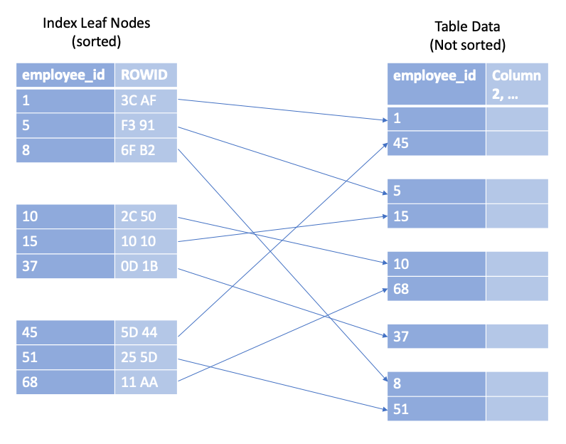
Each index entry consists of the indexed columns (column 2 in the diagram) and refers to the corresponding table row (ROWID). Unlike the index, this table data is stored in a heap structure so is not sorted at all.
The search tree (B-Tree) 🌴
The leaf nodes are not stored in a specific order - for example, consider book on programming with its index stored in the same manner; if you were searching the contents for ‘iteration’ and landed on ‘recursion’, it is by no means granted that ‘iteration’ is before ‘recursion’.

Databases overcome this by using a second structure to find the entries among the shuffled pages; a balanced search tree, or ‘B-tree’.
Like many trees in life, the B-tree has a root, branches and leaves (which we just covered). Each branch node entry corresponds to the biggest value in the respective leaf node, this hierarchy is applied backwards from all the leaf nodes until all the values are covered by a single node; the root node.
Once created, the database maintains this index automatically - adjusting it as necessary for every INSERT, UPDATE or DELETE statement and keeps the tree in balance.
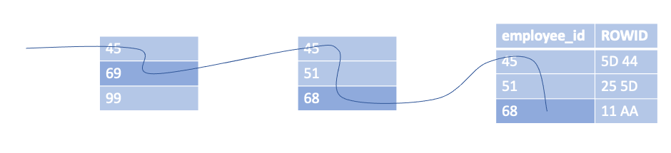
The diagram demonstrates how the tree is traversed to search for the key “68”. It starts at the root node, moving along until a value is greater than or equal to the search term, and then navigates to that branch node, and repeats. Eventually this traversal reaches the leaf node.
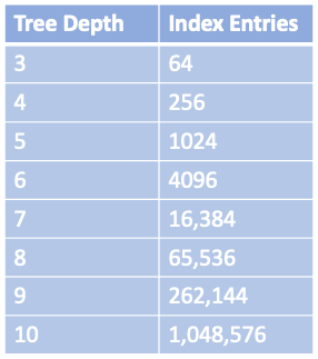
Tree traversal is a very efficient operation, it works almost instantly - even on a huge data set. Primarily because of the tree balance, and secondly because of the logarithmic growth of the tree depth. (In other words, the depth of the tree grows very slowly compared to the number of the leaf nodes). Real world indexes with millions of records only have a depth of four or five.
WHERE to begin… the Primary Key 🕵🏻♂️
The first ingredient of a slow query, is the WHERE clause. The WHERE clause defines the search condition of a SQL statement, and it is often phrased carelessly - causing the database to scan a large part of the index.
The primary key lookup is the simplest example of a WHERE clause. The primary key behaves as an index on the specified columns (in this case; the employee_id).
CREATE TABLE dbo.employees (
    employee_id   BIGINT         NOT NULL,
    first_name    NVARCHAR(1000) NOT NULL,
    last_name     NVARCHAR(1000) NOT NULL,
    date_of_birth DATE           NOT NULL,
    job_title     NVARCHAR(1000) NOT NULL,
    CONSTRAINT employees_pk PRIMARY KEY (employee_id)
);
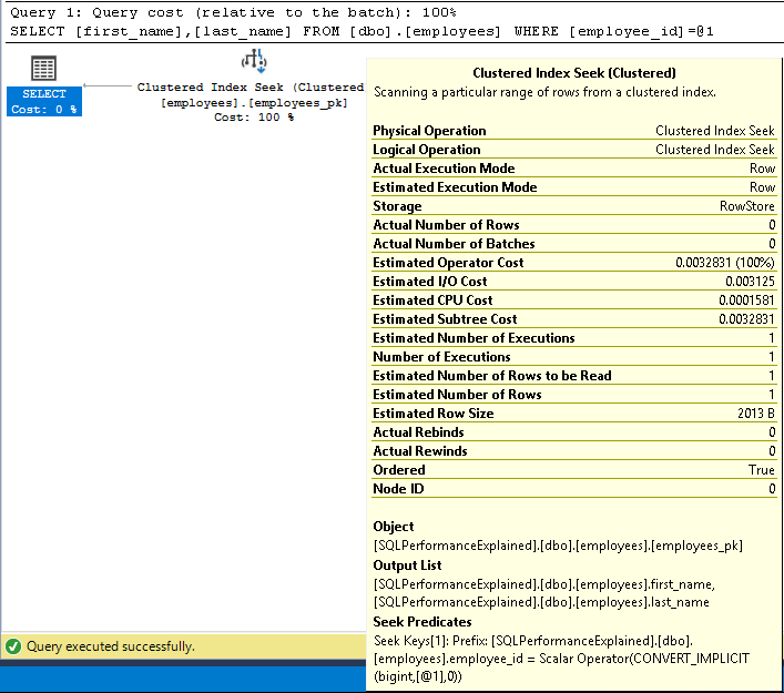
SELECT first_name, last_name
FROM employees
WHERE employee_id = 123
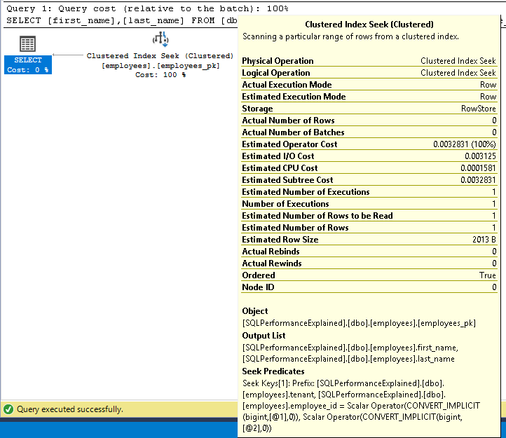
When running this query to fetch the employee’s name, the where clause cannot match multiple rows, as the primary key constraint ensures uniqueness of the employee_id values. When looking at the execution plan for this query, we can see an index seek was performed on the primary key; employees_pk.
Composite Primary Keys
A primary key can contain more than one column, sometimes called a concatenated, multi-column, or composite key. In a composite key column order is important, so it must be chosen carefully.
Consider the employee table from before, for demonstration let’s imagine we now want to make this table capable of storing employee information for multiple tenants, so we wish to add a tenant column and include it in the primary key.
CREATE TABLE dbo.employees (
    tenant        BIGINT         NOT NULL,
    employee_id   BIGINT         NOT NULL,
    first_name    NVARCHAR(1000) NOT NULL,
    last_name     NVARCHAR(1000) NOT NULL,
    date_of_birth DATE           NOT NULL,
    job_title     NVARCHAR(1000) NOT NULL,
);

CREATE CLUSTERED INDEX [employees_pk]
    ON [dbo].[employees] ([tenant], [employee_id])
When querying the data, we should now look to make use of the full primary key (ignoring the other reason to do this - ensuring tenant-safe reads!)
SELECT first_name, last_name
FROM employees
WHERE tenant = 1
AND employee_id = 123
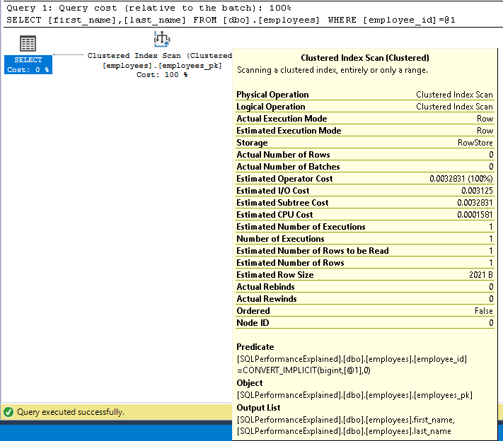
If running the original query, excluding tenant from the WHERE clause you can see the updated primary key is no longer used. Instead, a table scan occurs, and the database reads every row from the table data and compares them with the specified WHERE clause.
Columns in a composite key cannot be used arbitrarily, think back the tree traversal the of the B-Tree - since tenant is the first item in the primary key it must be specified in the WHERE clause or the index cannot be used.
A full table scan results in a query which may not appear to be expensive in a development environment, but as the table data grows this operation slows - and it is best to avoid finding out the hard way - in production 😱
We could of course add a second index to support the query and get round the table scan, but in this example it does not make sense to read from this table and not specify the tenant identifier - so this performance problem lies in the query and not the indexing.
Conclusion
Today I have described briefly how a Clustered Index is implemented, and how results are found using tree traversal. We have also covered a worked example of a composite primary key - and seen how column order can change the ability of the query optimiser to seek on a clustered index.


